#https://stackoverflow.com/questions/27934885/how-to-hide-code-from-cells-in-ipython-notebook-visualized-with-nbviewer
#cool code for a button to hide code
from IPython.display import HTML

HTML('''


<script>
code_show=true;
function code_toggle() {
 if (code_show){
 $('div.input').hide();
 } else {
 $('div.input').show();
 }
 code_show = !code_show
}
$( document ).ready(code_toggle);
</script>
<form action="javascript:code_toggle()"><input type="submit" value="Click here to toggle on/off the raw code."></form>
''')
import pandas as pd
import seaborn as sns
import matplotlib.pyplot as plt
import numpy as np
import tabulate
import statistical_tools as s_tools
import statsmodels.api as sm
from statsmodels.formula.api import glm
#plotting with seaborn
#https://cmdlinetips.com/2019/02/how-to-make-histogram-in-python-with-pandas-and-seaborn/

train = pd.read_csv("train.csv")
Analysis/Exploration 4 & Interaction testing:
Before we finally try modelling and predicting some of our data we will look into a few more of the factors we can test, alongside this we will test any 'interactions'. That is, we will see if some of the effect of a dependent variable has on our survival rate (Independent variable) is in fact influenced by another dependent variable.
Some additional variables that might be interedting (there are others we could engineer later such as the cabin code letter) will be family size:
- sibsp: number of siblings / spouses aboard the Titanic
- parch: number of parents / children aboard the Titanic
So again let's have a look whether there is interesting information about survival rates within these catgories
train.head()
train = train[train['SibSp'].notna()]
train = train[train['Pclass'].notna()]
train = train[train['Sex'].notna()]
First let's look at the distribution of values across these ordinal values:
print('Parch value counts')
print(train['Parch'].value_counts().sort_index())
print('SibSp value counts')
print(train['SibSp'].value_counts().sort_index())
We can see there is a poor spread of the data, that is, most of it is based in the 0 and 1 counts. This might mean that any insights from the other groups might be unreliably amplified by their low numbers. But we can still look into these.
prop_survived_parch = train['Parch'][train['Survived'] == 1].value_counts().sort_index()/train['Parch'].value_counts().sort_index()
prop_survived_parch = prop_survived_parch.fillna(0)

prop_survived_SibSp = train['SibSp'][train['Survived'] == 1].value_counts().sort_index()/train['SibSp'].value_counts().sort_index()
prop_survived_SibSp = prop_survived_SibSp.fillna(0)
#prop = train['Parch'].value_counts()/train['Parch'][train['Survived'] == 1]
def plot_prop(prop_series, x_axis, legend_name):
    df = pd.DataFrame({'proportion survived': prop_series,
                     'count': x_axis})


    sns.lineplot(x = 'count', y = 'proportion survived',  data=df, label=legend_name)
    #sns.distplot(,  kde=False,label='SibSp')
    #plt.ylim(0, 300)

    plt.legend(prop={'size': 12})
    #plt.title('All passengers ages vs survived passengers')
    plt.xlabel('Number of people')

    plt.ylabel('Proportions surviving')
    plt.title('Survival depending on family numbers')


plot_prop(prop_survived_parch, train['Parch'].value_counts().sort_index().index,  'Parch')
plot_prop(prop_survived_SibSp, train['SibSp'].value_counts().sort_index().index, 'SibSp')

We can definitely see some positive effects on survival, and that having a potentialy small size family ~1-3 people for siblings and spouses(Parch) may have some positive effects. And maybe a bit less for number of parents and children (SibSp) aboard. If we ignore the extreme numbers of people that have low amounts of data (i.e. 3 to 6 for parch and 3 to 8 for SibSp), we might be able to extract some information such as moving from 0 family to 1 or 2 has a positive effect on survival.
We might theorize that when children were being saved, parents were coming with them, or when there were bigger groups of siblings togethar they were more easily put in boats. Of course these factors may also have colinearity with other factors, for example richer higher 'Pclass' families might tend to have smaller families anyway? So let's get a quick look at that too.
Let's remember some previous analysis from below the survival rates for class:
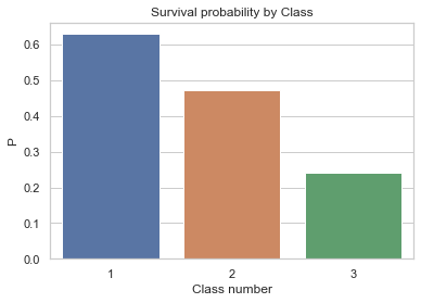
We can see that class has a strong effect on survival (we proved significance previously too). So we will look at the combination of class and Parch, but only using parch 0,1,2 as we saw more effect in these categories.
#https://seaborn.pydata.org/examples/grouped_barplot.html
sns.set(style="whitegrid")

# Load the example Titanic dataset
train_2 =train[((train['Parch'] ==0) | (train['Parch'] == 1) | (train['Parch'] == 2))]

# Draw a nested barplot to show survival for class and sex
g = sns.catplot(x="Pclass", y="Survived", hue="Parch", data=train_2,
                height=6, kind="bar", palette="muted");
#g.despine(left=True)
g.set_ylabels("survival probability");
plt.title('Survival depending on class and Parch (Siblings and spouse) numbers ');

We've got some interesting trends for class 1 and 2, where increasing from 0-3 family members has an increasingly positive effect on survival rate. However between classes there are vast difference and as I previously suggested, we will look for some possible interactions between them. We will just do this visually, and save any numerical tests for our modelling.
# code from previous workbook for getting seperate class values
def get_class_surv_prob(df):
    survived = df[df['Survived'] == 1]
    ones = df[df['Pclass'] == 1]
    ones_surv = sum(ones['Survived'] == 1)
    twos = df[df['Pclass'] == 2]
    twos_surv = sum(twos['Survived'] == 1)
    threes = df[df['Pclass'] == 3]
    threes_surv = sum(threes['Survived'] == 1)

    ones_prob = ones_surv/len(ones)
    twos_prob = twos_surv/len(twos)
    threes_prob = threes_surv/len(threes)
    return [ones_prob, twos_prob, threes_prob]

probs_0 =  get_class_surv_prob(train[train['Parch'] == 0])
probs_1 =  get_class_surv_prob(train[train['Parch'] == 1])
probs_2 =  get_class_surv_prob(train[train['Parch'] == 2])
avg =  get_class_surv_prob(train[((train['Parch'] ==0) | (train['Parch'] == 1) | (train['Parch'] == 2))])
df = pd.DataFrame({'Prop_surv':probs_0,
                      'Pclass': ['1','2','3']})
df2 = pd.DataFrame({'Prop_surv':probs_1,
                      'Pclass': ['1','2','3']})
df3 = pd.DataFrame({'Prop_surv':probs_2,
                      'Pclass': ['1','2','3']})
df_avg = pd.DataFrame({'Prop_surv':avg,
                      'Pclass': ['1','2','3']})

sns.lineplot(data=df, x='Pclass', y='Prop_surv',  label= 'Parch 0');
sns.lineplot(data=df2, x='Pclass', y='Prop_surv',  label= 'Parch 1');
sns.lineplot(data=df3, x='Pclass', y='Prop_surv', label= 'Parch 2');
sns.lineplot(data=df_avg, x='Pclass', y='Prop_surv', label= 'Parch 0, 1 & 2');
plt.title('Interaction affect between class and parch on survival');

We can see there is an interaction effect between Parch 1 and Parch 2 for 'Pclass 2'. Having 0 siblings or Spouses compared to 2 or 3 has a great affect on survival when people are from class 2 (middle class) as opposed to class 1 or 2.
This may make some sense, because we know the rich are likely better off regardless of their family - so the effect of Parch numbers is dimished in class 1. And maybe the 3rd class were both valued less and also in worse off cabins, so the effect of Parch on this class is also diminished. But the middle class were able to look out for each other, particularly a child with multiple siblings and a partner (we have found previously low ages and females have a significant increase in survival, so maybe having association to them helps also).
Seeing these results, and remembering how powerful an effect sex has on survival, I thought we would test some interactions between them too.
t1 = train['Sex'][train['Pclass'] == 1].value_counts()
t2 = train['Sex'][train['Pclass'] == 2].value_counts()
t3 = train['Sex'][train['Pclass'] == 3].value_counts()
print('Value counts class 1 \n{}\nclass 2 \n{}\nclass 3 \n{}'.format(t1, t2, t3))
#https://seaborn.pydata.org/examples/grouped_barplot.html
sns.set(style="whitegrid")

# Draw a nested barplot to show survival for class and sex
g = sns.catplot(x="Pclass", y="Survived", hue="Sex", data=train,
                height=6, kind="bar", palette="muted");
#g.despine(left=True)
g.set_ylabels("survival probability");
#plt.title('Survival depending on class and Parch (Siblings and spouse) numbers ')

probs_m =  get_class_surv_prob(train[train['Sex'] == 'male'])
probs_f =  get_class_surv_prob(train[train['Sex'] == 'female'])
avg =  get_class_surv_prob(train)

df = pd.DataFrame({'Prop_surv':probs_m,
                      'Pclass': ['1','2','3']})
df2 = pd.DataFrame({'Prop_surv':probs_f,
                      'Pclass': ['1','2','3']})
df3 = pd.DataFrame({'Prop_surv':avg,
                      'Pclass': ['1','2','3']})

sns.lineplot(data=df, x='Pclass', y='Prop_surv',  label= 'male');
sns.lineplot(data=df2, x='Pclass', y='Prop_surv',  label= 'female');
sns.lineplot(data=df3, x='Pclass', y='Prop_surv', label= 'avg');
plt.title('Interaction affect between class and sex on survival');

In this case we see a slightly similar effect, that class 1 has a very strong effect on survival, but also that being female prevent some of the detremental effect of droping down to class 2. However this effect was not enough to interact with and prevent a large drop in survival rate for class 3 in females.
Now some of these analyses could have been saved a bit by doing more catch all tests such as MANOVA for a number of our categories when compared against survival rate, however I feel that we have explored some of the data nicely here and also gotten some good practice in a number of these fundamental statistics tests and measures.
Next we will look to apply a basic model.